
III. Molecular Dynamics Simulations with Stochastic Boundary Conditions:
Application to the study of echistatin, an RGD containing snake toxin.
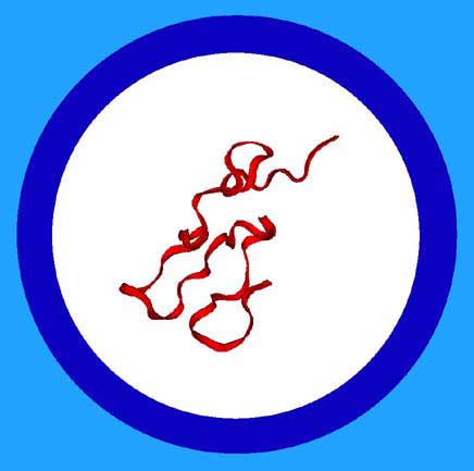
In this exercise, a simulation of the protein echistatin is done in explicit water using stochastic boundary conditions. Stochastic boundary conditions are often used in the simulation of spherical systems and it is often less computationally demanding than using periodic boundary conditions. In the present example, the entire echistatin protein from Exercise 1 is solvated by a sphere of explicit water. The sphere has a radius of 30Å and includes approximately 6800 water molecules. The sphere is divided into two regions (see figure below); an inner reaction region and an outer buffer region. In the reaction region (white), the molecular dynamics simulations are done in the conventional way, e.g. using Newton’s equations of motion. In the buffer region (dark blue), the molecular dynamics are treated explicitly using the Langevin equations of motion (see below). This hybrid method couples the water molecules in the buffer region to a heat bath (light blue) which keeps the system at thermal equilibrium. A spherical boundary potential is employed to maintain the correct average distribution of water molecules and to prevent water from escaping into the vacuum. The stochastic boundary approach removes water molecules that are far from the area of interest (in this case the protein echistatin) thus reducing the number of explicit water molecules in the simulation while still including, in an approximate way, their effect on the molecules in the reaction region.
The Langevin equation:
In the Langevin equation, the force on the particle is divided into three components (see the equation below). The first component is the interatomic force, Fi{xi(t)}, due to the interaction between the atoms in the system, for example, between two atoms of a protein. This is the same force used in Newton’s equation of motion. The second component is a frictional force which describes the drag on the particle due to the solvent. The magnitude of the drag is related to the friction coefficient, gi. The third component, Ri(t), is the random or stochastic force due to thermal fluctuations of the solvent. The solvent is not explicitly represented but its effects on the explicit atoms comes from the frictional and random forces. When the frictional and random forces are zero, the Langevin equation reduces to Newton’s equation of motion.

The Langevin equation generates classical Brownian dynamics which describes the motion of a particle under the influence of random collisions with the surrounding solvent.
The present approach is a hybrid molecular dynamics - Brownian dynamics method where the reaction region undergoes conventional Newtonian dynamics but the water molecules in the buffer region undergo Brownian dynamics. These water molecules interact explicitly with the protein atoms and the water molecules in the reaction and the buffer regions; the effect of the friction coefficient and the random force approximate the effects of the water that would be outside of the sphere. This approach reduces the number of explicit water molecules in the simulation while still including, in an approximate way, their effect on the molecules in the reaction and buffer regions.
For a more detailed discussion of the Langevin equation and the stochastic boundary method, see the following references.
References
Allen, M. P. and Tildesley, D. J. (1989). Computer Simulation of Liquids. Oxford, Oxford Univ Press.
Brooks, C. L., Karplus, M. and Pettitt, B. M. (1988). Proteins: A Theoretical Perspective of Dynamics, Structure, and Thermodynamics. Advances in Chemical Physics. John Wiley & Sons.
Brooks, C. L. I. and Karplus, M. (1989). Solvent Effects on Protein Motion and Protein Effects on Solvent Motion. J. Mol. Biol. 208: 159 - 181.
Leach, A. R. (1997). Molecular Modelling : Principles and Applications. Addison-Wesley Pub. Co.
Stote, R. H., Dejaegere, A. and Karplus, M. (1997). Molecular Mechanics and Dynamics Simulations of Enzymes. Computational Approaches to Biochemical Reactivity. Netherlands, Kluwer Academic Publishers.
|
|
Procedure
The procedure to carry out a molecular dynamics simulation of a protein in explicit solvent using the stochastic boundary conditions is outlined below. Be aware that the explicit treatment of the solvent is significantly more CPU intensive than the implicit treatment used in the vacuum simulations (Exercise 1).
Preparation
-
Generation of the PSF for a biomolecule
-
Energy calculation
-
Energy minimization
Dynamics in water, solvation sphere:
-
Solvation of the biomolecule by a solvent sphere
-
Equilibrating the water molecules around the fixed protein
-
Heating - Equilibration- Production of the entire system
-
Analysis of results
Note that the Preparation steps are the same as in the previous exercises; see Exercise 1 for detailed instructions.
|
Download the following input files:
The first step is to prepare the protein molecule as was done in Exercise 1. Do this before continuing this tutorial.
After the initial preparation, the water is added to the system. The CHARMM commands for solvating the protein by a sphere of water are given in the file named solvate.inp; the coordinates for a 37Å radius water sphere are given in the file sphere37.crd.
* Solvate1.inp
* Solvate the protein Echistatin with a water sphere
*
! Read in Topology and Parameter files
open unit 1 card read name top_all22_prot.inp
read RTF card unit 1
close unit 1
open unit 1 card read name par_all22_prot.inp
read PARA card unit 1
close unit 1
! Read PSF file
open unit 1 card read name 2ech.psf
read psf card unit 1
! Read in energy minimized coordinates
open unit 1 read formatted name 2ech-mini.pdb
read coor pdb unit 1
close unit 1
! To Begin, translate the system to insure it is at the origin }
define origin select all end
! { find the centre of the reaction region }
coordinate statistics select ( origin ) end
! { make this point the origin }
coordinate translate xdirection -?XAVE ydirection -?YAVE zdirection -?ZAVE
! { verify }
coordinate statistics select ( origin ) end
|
|
The topology and parameter files are first read into CHARMM, followed by the psf and coordinate file for the energy minimized protein generated during the preparation stage. The protein is centered at the origin using the sequence of commands shown above in blue. The values of XAVE, YAVE, ZAVE define the geometric center of the protein and are determined by the coordinate statistic command. The entire protein is then translated such that the center coincides with the origin; the command for this operation is coordinate translate. If one is interested in solvating a smaller region of the protein, the center of this region (an active site, for example) should be translated to the origin.
Once centered, the protein is solvated in the following manner: a sufficiently large sphere or box of pre-equilibrated water is read into CHARMM; a segment ID is generated for the water and the coordinates are appended to the existing protein coordinates already in CHARMM. The command for this operation are shown below.
! Read in water sphere sequence
open unit 1 read formatted name sphere37.crd
read sequence coor unit 1
rewind unit 1
! Generate new segment for the water sphere
generate bulk noangle nodihedral
! Read water sphere coordinates
read coor card unit 1 append
close unit 1
|
The keywords noangle and nodihedral in the above generate command specify the exclusion of angle and dihedral angle energy terms in the potential function for the water molecules. The default water molecule in the CHARMM force field is closely related to the TIP3P water molecule (Jorgensen et al. 1983, J. Chem. Phys. 79: 926; Neria et al 1996, J. Chem. Phys. 105: 1902); this model contains three particles, the oxygen and two hydrogen. The geometry of the molecule is defined by the two oxygen - hydrogen bond distance and the hydrogen-hydrogen distance. This particular water model is rigid, there is no internal flexibility.
The next set of commands remove those water molecules which overlap the protein; the delete command which a specific set of atom selections is used. An overlapping water molecule is one which is found in a radius of 2.8Å from a protein atom. The second delete command removes those water molecules which lie outside the 30Å sphere.
! Center the water sphere
coordinate orient noro select segid bulk end
! Delete waters which overlap with protein }
delete atom sort -
select .byres. (segid bulk .AND. type oh2 .and. -
((.not. (segid bulk .OR. hydrogen)) .around. 2.8)) end
! Delete all water beyond the outer cutoff
delete atom sort -
select .byres. ( .not. ( point 0. 0. 0. cut 30.0) -
.and. ( segid bulk .AND. type oh2 ) ) end
! End of solvation of system
|
The remainder of the input file (not shown) writes out the resulting PSF and PDB file for the solvated protein.
Execute this command file using the CHARMM program by typing the following command at the UNIX prompt; the job should take less than a minute to run.
charmm < solvate.inp > solvate.out
Do an ls in your directory to see the new files corresponding to the psf file and the pdb file of the protein-water system. Using a graphics program of your choice, look at the resulting coordinate file to visually ensure that the protein is properly solvated.
You can see the output file here -->solvate.out
Look through the output file to find how many waters were deleted in order to accommodate the protein.
ii) Equilibration of the water around a fixed protein
The next input file (equilibrate-water.inp) sets up a molecular dynamics simulation which equilibrates the water around the protein. This is necessary because the water configuration that was used to solvate the protein corresponds to equilibrated pure water. The water molecules that remain in the system are now in a different environment, i.e., surrounding a protein molecule. Therefore, before starting a simulation of the protein-water system, it is best to first allow the water molecules to rearrange in response to the presence of the protein. This will result in a smoother initiation of the protein-water simulation.
The water molecules are kept within the sphere through the use of a boundary potential (Brooks III and Karplus 1983, J. Chem. Phys. 79, 6313). The boundary potential is precalculated for a sphere of a given size; boundary potentials for spheres up to 25Å in radius are included in the CHARMM distribution (in the support/bpot subdirectory). In the present tutorial, a sphere of 30Å is used to solvate the protein, the data for the boundary potential is given in the file bp30.dat. The commands for setting up the boundary potential are shown below.
! Read in solvent boundary potential
OPEN UNIT 1 READ FORMatted NAME bp30.dat
SBOUnd READ UNIT 1
CLOSE UNIT 1
SBOUND SET XREFerence 0.0 YREFerence 0.0 ZREFerence 0.0 -
ASSIgn 1 SELEct ( ( RESName tip3 .AND. TYPE oh2 )) END
|
The boundary potential data is read in into CHARMM using the SBOUnd READ command and it is set up internally using the SBOUND SET command. When setting up the boundary potential, it is necessary to define the origin of the potential; in the present example, as in most cases, the origin of the boundary potential will coincide with the center of the water sphere. The boundary potential is then assigned to act on all oxygen atoms belonging to the TIP3P water. The boundary potential is a function of the distance between the oxygen atom and the origin as defined in the SBOUND SET; it is near zero until one reaches the outer limit of the sphere.
As explained in the introduction section of this exercise, the water sphere is divided into two regions, the reaction region, where the dynamics is carried using the conventional equations of motion, and the buffer region, where the molecular dynamics are calculated using the Langevin equation of motion. In the next segment of input file, the dynamics simulation of the water with the fixed protein is set up. The Langevin friction coefficients for the water oxygens are defined using the SCALAR command. The value of the friction coefficient used here was determined from an earlier simulation of pure water (Brünger, et al. 1984, Chem. Phys. Lett. 30, 495). The protein prot is then constrained to its initial position using the CONS FIX command.
! { Langevin friction coefficients }
SCALAR FBETa SET 0.0 SELEct ( ALL ) END
SCALAR FBETa SET 62.0 SELEct ( RESName TIP3 .AND. TYPE oh2 ) END
CONS FIX PURGe SELEct segid prot END
MINImize SD nstep 100 nprint 1 inbfrq 10 ihbfrq 0
SHAKE BONH TOLErance 1.0e-6 PARAMeter

DYNAmics Leap LANGevin STRT -
NSTEp 500 TIMEstep 0.002 -
ISEED 918237912 -
NPRInt 100 IPRFrq 250 -
ILBFrq 5 RBUFfer 25 TBATh 300 -
IUNCRD -1 NSAVC 00 IASORS 1 -
FIRStt 300 -
INBFrq 10 IHBFrq 0 WMIN 1.2
! Write Coordinates
OPEN UNIT 1 WRITe FORMatted NAME scr/sbmd2.pdb
WRITe COORdinate CARD UNIT 1
* COORdinates
* INITIAL SOLVENT EQUILIBRATION: SOLUTE FIXED
*

STOP
|
|
Prior to starting the simulation, a short energy minimization using the steepest descent algorithm is done to remove any strong van der Waals contacts between the water and the protein. The SHAKE algorithm is used to constrain all hydrogen-heavy atom bond lengths to their default values. This is done because simulating the high frequency of the hydrogen-heavy atom bond vibration would necessitate the use of a very short time step. This, in turn, would lead to a very time consuming simulation.
We finally arrive at the command for starting the molecular dynamics simulation. The keywords are essentially the same as in the previous exercise with several exceptions. Because we are doing is a stochastic boundary simulation, we use the Langevin algorithm for the molecular dynamics simulation rather than the Verlet algorithm. In both cases the Leap frog algorithm is used to integrate the equations of motion. There are several additional keywords that one must use for the Stochastic boundary simulation. These include
-
The LANGevin keyword specifies the Langevin method should be used for the simulation.
-
ILBFrq specifies the number of steps between the update of the list of water molecules in the Langevin buffer region. Since water molecules can pass between the buffer region and the reaction region, it is necessary to periodically update an internal list which specifies which waters should be treated by conventional dynamics and which should be treated by Langevin dynamics. In the current example, the list update is done every 5 time steps.
-
RBUFfer: This parameter defines the division between the reaction region and the buffer region is defined. This parameter is the inner radius of the Langevin buffer region; in the current example, this inner radius is 25Å, so the Langevin region is between 25Å and 30Å.
-
TBATh: This is the temperature of the Langevin thermal bath; in the current example the bath temperature is 300K.
The simulation is done for 10000 time steps (NSTEp) and the time step is 0.002ps (TIMEstep).
iii) Heating Equilibration and Production runs
Once the protein has been solvated and the surrounding water equilibrated around the protein, all constraints on the protein are removed and the system is prepared for the protein dynamics. In general, these steps are the same as those carried out in the vacuum simulations, e.g., the system is slowly heated then equilibrated at the desired temperature before continuing with the production phase. The next three input files (heat.inp, equilibrate.inp and run1.inp) execute these three stages.
Compare these input files to the corresponding ones from of Exercise 1. Notice that they do essentially the same procedure with the exception that in each of the present input files, the boundary potential is step up and the friction coefficients defined. Execute them sequentially using CHARMM.
Exercise: Using run1.inp as a template, modify the input file to run the next segment of the simulation (run2.inp).
Analysis
In this section, we will carry out the same analysis as was done for the vacuum simulations after some modification of the input files.
1. After carrying out the molecular dynamics simulation of the protein in water, extract the energies that were printed in the output files (Follow the same procedure used in the previous exercises using the UNIX grep command)
grep 'DYNA>' run1.out > run1.data
Using the awk script energy.awk, calculate the mean total energy and the fluctuations.
How does the quality of the simulation compare to the quality of the previous simulations based on these criterion? {Answer, the fluctuations in the stochastic boundary molecular dynamics are usually slightly larger than in the vacuum and periodic boundary dynamics simulation}
2. Calculate the average structure of the protein from the trajectory and the calculate the dihedral angle time series of the backbone dihedral angles of the RGD segment.
Using the CHARMM command file md_anal.inp, calculate the average structure from the simulation. See Exercise 1 for a complete description of this input file.
Using the input file dihedral.inp, calculate the f24 and y24 of Gly24 and f25, y25 of Asp25; what values do you find? {my answer, 173.6, -80.2, -108.5, -60.8, respectively.} Calculate the values of these dihedral angles in the original PDB coordinate file {my answer, -52.9, -51.2, -128.9, -42.7, respectively}
Plot the time dependent behavior of the four backbone dihedral angles of the RGD sequence (f24 and y24 around the Ca of residue 24 (Gly) and f25, y25 around the Ca of residue 25 (Asp)). The time series were calculated in md_anal.inp using the CORRel facility. Are there any significant conformational changes of the RGD sequence in the time span of the simulation? Relative to the initial structure? time series graphic
Note: your dihedral angle values will probabaly differ from the values given above due to slightly different trajectories which result from doing the calculations on different platforms.
|